FORECAST EARLIER. DECIDE BETTER.

Time Series
Foundation ModelAI that reads your data.
And looks ahead.

A Time Series Foundation Model is an AI model pretrained on many time series. It takes a history of sales, energy use or sensor readings and estimates future values, together with their uncertainty.

It forecasts numbers. To help you act earlier.

Find your use case ↓How it works ↗

An ICAREX guide · Updated 26 October 2026

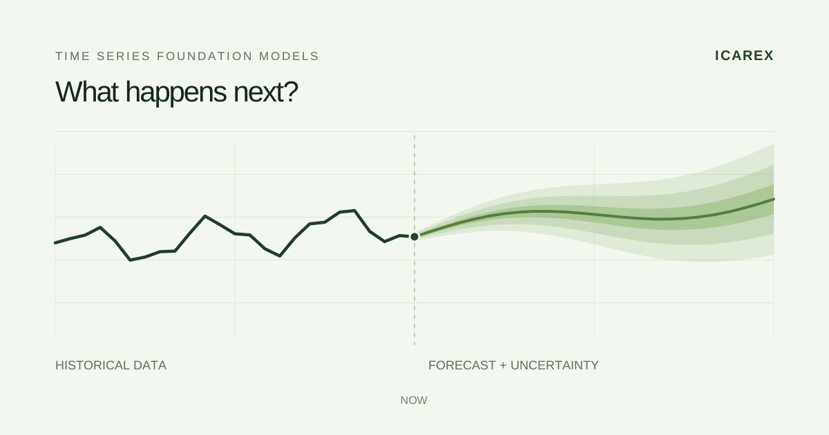
Historical data and a future forecast with an uncertainty band. — INPUTYour data over timeOUTPUTFuture values and uncertainty

Timestral, by Mistral AI, is one of these models. It reads several variables together and can run forecasts on a CPU, without a dedicated GPU.[1]

01 / HOW IT WORKS

From past data
to the next steps.

A time series is a sequence of measurements over time: daily sales, temperature every minute, power use every quarter of an hour. The model forecasts what comes next.

01
Give it a history.
You can start from a CSV: dates, times and one or more variables. Software passes the numbers to the model.
02
Choose how far ahead to look.
The time step matches your data: 4 steps of 15 minutes cover the next hour.
03
See the uncertainty too.
For each step: a median, a lower value and an upper value. You can see the forecast’s uncertainty too.

Try it: a plant’s power demandkW

Data everyFuture steps

4 × 15 min = 1 hour

HistoryMedianLower–upper band

Simulated data: the chart illustrates the process; it does not run Timestral.

See the CSV and every forecast value


Date and time	Step	Lower P10	Median P50	Upper P90

The CSV shows the last four rows. The selected time step must match the prepared data.

The future is more than one number. The P10–P90 band represents expected 80% coverage at each step, to be checked. These are not guaranteed minimum and maximum values; the median is not their average.[2][6]

02 / WHERE IT CREATES VALUE

Which of these problems
sounds familiar?

Stock, equipment, energy. Choose your field to see the data, the forecast and the decision it can change.

RETAIL / DEMAND AND REPLENISHMENT

How much will each product sell across my stores?

Buy too much and you have stock to mark down. Buy too little and you lose sales. Demand forecasting helps find a balance.

For teams managing assortments and purchasing across stores or channels.

THE DATA YOU START WITH

Sales by product and storeStock and availabilityPrices and promotionsCalendar and seasonality

THE FORECASTExpected demand by product and store, week by week. Here we look 12 weeks ahead.

THE DECISIONDecide how much to order and where to allocate stock, considering inventory, deliveries and supplier lead times.

One product, one store · weekly salesunits / week

SIMULATED DATA · An example, not a forecast run by Timestral.

HistoryMedianLower–upper band

Choose a week to inspectWeek +4

Week +4

Lower · P10120 units

Median · P50160 units

Upper · P90210 units

WHERE IT CAN HELP

Less idle stock

Purchasing aligned with demand.

Fewer markdowns

Surplus spotted earlier.

Fewer lost sales

Products available where needed.

Let’s discuss your inventory ↗

Let’s look at your data and the decision you want to improve.

How do we measure the inventory benefit?

Start with selected categories and stores. Simulate orders using the new forecasts and compare them with your current method under the same delivery constraints. Then validate in practice.

Measure inventory, stockouts, markdowns and margin. Cash released from inventory is not an annual saving.

Read sales alongside stock levels: a sold-out product may hide unmet demand. This comparison considers one week at a time. A real replenishment plan must also cover later weeks and respect supplier constraints.

Forecasts support decisions. Benefits depend on the actions taken and must be verified after costs. These examples are not customer results.

03 / WHY TIMESTRAL

A reusable model.
No GPU required.

Timestral comes pretrained. You can try it on new histories and run it on a server’s CPU. This can reduce initial setup work and infrastructure costs.[1]

Zero-shot

An initial forecast on new data, without task-specific training. Accuracy needs checking in your context.

Several signals together

Temperature, pressure and vibration from the same pump: this is what multivariate means.

It uses your plans

Scheduled shifts, stops and promotions can be supplied as data: known-future covariates.

From 5 to 209 million parameters. Four sizes to choose from based on accuracy, memory and forecast volume.

What might it cost? Open the calculator.

Mistral reports 17 ms for 5M and 113 ms for 209M: an 8-thread CPU, 3 weeks of 15-minute history and a one-day forecast. These are vendor measurements, not a benchmark on the server below.[1]

A REAL SERVER. EDITABLE ASSUMPTIONS.

What does it cost to run forecasts?

Choose a model and change the number of calls. Compare the value of compute time with the cost of a server available all month.

Model calls / dayTime per call (ms)Whole server (€/hour)

96,000 calls/day is an example: 1,000 machines, one call every 15 minutes. One call returns all requested future steps; each forecast point is not a separate call.

Hetzner CCX33 · 8 vCPU · 32 GB RAM

Rate: €0.2219/hour. Monthly cap: €138.49. Germany/Finland, excluding VAT and IPv4. Price list checked on 26 October 2026. You can enter another server’s rate.

See the official price list ↗[11][12]Apply Hetzner’s €138.49 monthly cap

Cost of one server available all month

Value of time spent computing onlyA theoretical compute allocation, not the server bill.

Average server cost / 1,000 calls

Verified price; performance still needs verification. The 17/113 ms timings are Mistral measurements on an 8-thread CPU, not a test on this Hetzner. Assumptions: 30 days, sequential calls at constant latency, whole server occupied during each call. Excludes data loading, model startup, other workloads, integration, monitoring, staffing and any licence fees.[1]

The formulas, with no hidden steps

Compute hours = calls/day × 30 × milliseconds / 3,600,000. Time value = compute hours × €/hour. Server cost = 720 × €/hour, capped at €138.49 if the Hetzner cap is enabled. Average cost per 1,000 calls = server cost / monthly calls × 1,000. Changing the rate automatically disables the Hetzner cap.

THE NEXT STEP

What if we tried it
on your use case?

Tell us about a decision you would like to make earlier. We’ll look at your data, the forecast you need and how to test whether it is worthwhile.

Explore my use case ↗

A concrete problem. Your data. A benefit to test.

The questions that matter.

Does zero-shot mean no data is needed?

No. You need historical data. Zero-shot means using the model on a new series without first training it on that task. If a machine changes, you can try its history with the same model; insufficient results may require adaptation.[1]

What changes compared with ARIMA?

ARIMA is usually fitted to a single series. A foundation model starts from broad, reusable pretraining. Models working across several series already existed: the innovation is the general-purpose starting point, not forecasting itself. Comparison with your current method remains essential.[1][4][5]

How do you provide a planned stop or promotion?

As a variable linked to future dates, not a chat note. A scheduled shutdown, for example, helps the model expect lower power use. These inputs are called known-future covariates. Weather forecasts can also be inputs, but remain uncertain.[2]

Include the 14:00–16:00 shutdown

Simulated example: the dashed line shows example measurements and the green band the forecast.

How can I tell whether forecasts are reliable?

Test them on past data using only information available at the time. Measure error and interval reliability, compare with the current method and simulate the resulting decisions. A more accurate chart matters if it changes an operational or financial outcome.[6]

Is Timestral the only model of this kind?

No. Other families include Amazon’s Chronos and Google’s TimesFM. Timestral is trained first on synthetic series, then on real and synthetic data. For a project, the choice should follow results on your data, not just published benchmarks.[1][7][8]

Can a business use it? What is the license?

The code uses Apache 2.0; model weights use a Modified MIT license. For the 209M checkpoint reviewed, global consolidated revenue above US$20 million in the preceding month requires a commercial agreement with Mistral. Check the license for your chosen version.[9]

Sources and references

By ICAREX. Sources reviewed on 26 October 2026. Educational examples and simulations created by ICAREX.

Mistral · Introducing Timestral · 15.10.2026 ↗
Training, CPU and vendor-reported launch results.
Mistral · Repository Timestral ↗
Inputs, quantiles, covariates, weights and inference.
Mistral · Model card 209M ↗
Architecture, context and benchmark table.
Hyndman & Athanasopoulos · Dynamic regression ↗
External regressors and models with ARIMA errors.
Hyndman & Athanasopoulos · Vector autoregressions ↗
Models using multiple variables already existed.
Hyndman & Athanasopoulos · Forecasting toolbox ↗
Prediction intervals, metrics and time series validation.
Amazon Science · Chronos-2 ↗
Another multivariate foundation model with covariates.
Google Research · TimesFM-3 · 31.08.2026 ↗
The TimesFM family and its move to multivariate forecasting.
Mistral · Timestral-209M · Modified MIT License ↗
Model weights license for the 209M checkpoint.
TypeSafe · System One ↗
The parallel with models for structured answers and choices.
Hetzner · Cloud price list · 15.06.2026 ↗
CCX33 rate and monthly cap, excluding VAT and IPv4.
Hetzner · General Purpose ↗
CCX33 specifications, dedicated CPUs and billing terms.
Mistral · Brand assets ↗
Official brand mark, used to identify the developer.

What would you like to anticipate?

A few lines about the problem you want to solve are enough. We’ll help identify the data you need and where to start.

Or email us directlyinfo@icarex.ai

Time Series
Foundation ModelAI that reads your data.
And looks ahead.

From past data
to the next steps.

Give it a history.

Choose how far ahead to look.

See the uncertainty too.

Which of these problems
sounds familiar?

How much will each product sell across my stores?

Less idle stock

Fewer markdowns

Fewer lost sales

Could this pump move outside its operating limits?

More time to act

Fewer urgent interventions

More stable processes

How much energy will my plants produce tomorrow?

Fewer costly imbalances

Clearer risk

Coverage across more plants

A reusable model.
No GPU required.

Zero-shot

Several signals together

It uses your plans

What does it cost to run forecasts?

What if we tried it
on your use case?

The questions that matter.

What would you like to anticipate?

Time SeriesFoundation ModelAI that reads your data.And looks ahead.

From past datato the next steps.

Give it a history.

Choose how far ahead to look.

See the uncertainty too.

Which of these problemssounds familiar?

How much will each product sell across my stores?

Less idle stock

Fewer markdowns

Fewer lost sales

Could this pump move outside its operating limits?

More time to act

Fewer urgent interventions

More stable processes

How much energy will my plants produce tomorrow?

Fewer costly imbalances

Clearer risk

Coverage across more plants

A reusable model.No GPU required.

Zero-shot

Several signals together

It uses your plans

What does it cost to run forecasts?

What if we tried iton your use case?

The questions that matter.

What would you like to anticipate?

Time Series
Foundation ModelAI that reads your data.
And looks ahead.

From past data
to the next steps.

Which of these problems
sounds familiar?

A reusable model.
No GPU required.

What if we tried it
on your use case?